Heteroskedasticity: Definition, Causes, and Implications

Heteroskedasticity: Definition, Causes, and Implications

Heteroskedasticity is a statistical term that refers to the unequal variability of errors or residuals in a regression model. In simpler terms, it means that the spread or dispersion of the residuals is not constant across the range of values of the independent variable(s).

Heteroskedasticity can lead to biased and inefficient estimates of the regression coefficients. This means that the estimated coefficients may not accurately represent the true relationship between the independent and dependent variables. In addition, heteroskedasticity can affect the statistical significance of the coefficients and lead to incorrect inferences.

Causes of Heteroskedasticity

There are several potential causes of heteroskedasticity. One common cause is the presence of outliers or extreme values in the data. These outliers can have a disproportionate impact on the variability of the residuals. Another cause is the omission of important variables from the regression model. If these omitted variables are correlated with the independent variables, they can lead to heteroskedasticity.

Furthermore, heteroskedasticity can also be caused by the nature of the data itself. For example, financial data often exhibits heteroskedasticity due to the inherent volatility and uncertainty in the markets. Other factors such as measurement errors, data transformation, and model misspecification can also contribute to heteroskedasticity.

Impact of Heteroskedasticity on Portfolio Management

Heteroskedasticity can have significant implications for portfolio management. It can affect the estimation of risk and return parameters, leading to inaccurate portfolio optimization and asset allocation decisions. Inaccurate risk estimates can result in suboptimal portfolio diversification and increased exposure to risk.

Moreover, heteroskedasticity can affect the performance evaluation of investment strategies. If the variability of returns is not properly accounted for, it can lead to biased performance measures and misjudgment of investment performance. This can have serious consequences for investors and portfolio managers.

Identifying and Testing for Heteroskedasticity

There are several statistical tests that can be used to detect heteroskedasticity. One commonly used test is the Breusch-Pagan test, which tests for the presence of heteroskedasticity based on the relationship between the squared residuals and the independent variables. Other tests include the White test, the Goldfeld-Quandt test, and the Park test.

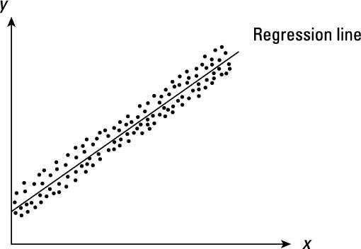
In addition to statistical tests, graphical methods such as scatterplots of the residuals against the independent variables can also be used to identify heteroskedasticity. If the scatterplot exhibits a cone-like shape or a clear pattern, it may indicate the presence of heteroskedasticity.

Addressing Heteroskedasticity in Portfolio Management

Another approach is to transform the data using mathematical functions, such as logarithmic or square root transformations, to stabilize the variance of the residuals. However, it is important to note that these transformations may alter the interpretation of the coefficients and may not always be appropriate.

Furthermore, portfolio managers can also consider using alternative risk measures, such as Value at Risk (VaR) or Conditional Value at Risk (CVaR), which are less sensitive to heteroskedasticity. These risk measures provide a more robust assessment of downside risk and can help in making more informed portfolio decisions.

Heteroskedasticity is a statistical term that refers to the unequal variance of errors or residuals in a regression model. In simpler terms, it means that the variability of the dependent variable is not constant across all levels of the independent variable(s).

When heteroskedasticity is present in a regression model, it violates one of the key assumptions of ordinary least squares (OLS) regression, which assumes that the errors have constant variance (homoscedasticity). This can lead to biased and inefficient estimates of the regression coefficients, making it difficult to draw accurate conclusions from the analysis.

There are several reasons why heteroskedasticity may occur in a regression model. One common cause is the presence of outliers or extreme values in the data. These outliers can have a disproportionate impact on the variability of the dependent variable, leading to heteroskedasticity.

Another cause of heteroskedasticity is the omission of relevant variables from the regression model. If important variables are left out of the analysis, the remaining variables may not fully capture the variability in the dependent variable, resulting in heteroskedasticity.

Heteroskedasticity can also be caused by the nature of the data itself. For example, financial data often exhibits heteroskedasticity due to the inherent volatility and uncertainty in the markets. Similarly, time series data may exhibit heteroskedasticity due to changing economic conditions or other factors.

The implications of heteroskedasticity on portfolio management can be significant. If heteroskedasticity is present in the data used to construct a portfolio, the risk estimates and performance measures may be biased or inaccurate. This can lead to suboptimal portfolio allocation decisions and potentially higher levels of risk.

If heteroskedasticity is detected, there are various techniques and models that can be used to address it. One common approach is to use robust standard errors in the regression analysis, which adjust for heteroskedasticity and provide more accurate estimates of the regression coefficients.

Another approach is to transform the data or use weighted least squares regression, which can help mitigate the impact of heteroskedasticity. Additionally, advanced modeling techniques, such as generalized autoregressive conditional heteroskedasticity (GARCH) models, can be used to explicitly model and account for heteroskedasticity in the data.

Causes of Heteroskedasticity

Heteroskedasticity refers to the unequal variability of errors in a regression model. In other words, it occurs when the variance of the error term is not constant across all levels of the independent variables. There are several causes of heteroskedasticity that can affect the reliability and accuracy of statistical models.

1. Outliers

Outliers are extreme observations that deviate significantly from the rest of the data. When outliers are present in the data, they can introduce heteroskedasticity by increasing the variability of the error term. These outliers may be caused by measurement errors, data entry mistakes, or other factors that result in extreme values.

2. Missing Variables

3. Functional Form Misspecification

Heteroskedasticity can also arise from misspecification of the functional form of the regression model. If the relationship between the dependent variable and the independent variables is not correctly specified, it can result in heteroskedasticity. For example, if a linear model is used to analyze data that follows a non-linear pattern, the errors may exhibit heteroskedasticity.

4. Time-Varying Variance

Time-varying variance occurs when the variability of the error term changes over time. This can be caused by various factors such as changes in market conditions, economic cycles, or other time-dependent variables. When the variance of the error term is not constant over time, it violates the assumption of homoscedasticity and leads to heteroskedasticity.

Impact of Heteroskedasticity on Portfolio Management

One of the main impacts of heteroskedasticity on portfolio management is the distortion of risk measures. Traditional risk measures, such as standard deviation and beta, assume constant variances across all observations. However, in the presence of heteroskedasticity, these measures may underestimate or overestimate the true risk of an investment.

Underestimating risk can lead to the inclusion of overly risky assets in a portfolio, potentially exposing investors to higher levels of volatility and losses. Overestimating risk, on the other hand, can result in the exclusion of potentially profitable assets, leading to missed opportunities for portfolio diversification and returns.

Heteroskedasticity can also impact portfolio optimization techniques. Traditional mean-variance optimization models assume constant variances, which may not hold true in the presence of heteroskedasticity. As a result, the optimal portfolio weights calculated using these models may not accurately reflect the true risk-return tradeoff.

To address the impact of heteroskedasticity on portfolio management, various techniques can be employed. One approach is to use robust estimation methods, such as weighted least squares or generalized least squares, which account for heteroskedasticity in the regression model. These methods adjust the standard errors and coefficient estimates to provide more accurate risk assessments.

Another approach is to employ portfolio optimization models that explicitly account for heteroskedasticity. These models incorporate measures of conditional volatility, such as GARCH (Generalized Autoregressive Conditional Heteroskedasticity), to capture the time-varying nature of risk. By considering the changing volatility patterns, these models can generate more robust and efficient portfolios.

Overall, the impact of heteroskedasticity on portfolio management highlights the importance of accurately assessing and addressing risk. By recognizing and accounting for the presence of unequal variances, investors can make more informed decisions and construct portfolios that better align with their risk preferences and investment objectives.

Identifying and Testing for Heteroskedasticity

Heteroskedasticity refers to the phenomenon where the variance of the error term in a regression model is not constant across all levels of the independent variables. It can have significant implications for portfolio management as it violates the assumptions of classical linear regression models.

Identifying heteroskedasticity is an important step in portfolio management. There are several graphical and statistical methods available to detect heteroskedasticity:

1. Graphical Methods:

Another graphical method is the time series plot of the residuals. If the plot shows a pattern of increasing or decreasing variability over time, it suggests the presence of heteroskedasticity.

2. Statistical Tests:

There are several statistical tests available to formally test for heteroskedasticity. One commonly used test is the Breusch-Pagan test. It involves regressing the squared residuals on the independent variables and testing the significance of the coefficients. If the coefficients are significantly different from zero, it indicates the presence of heteroskedasticity.

Another test is the White test, which is a generalization of the Breusch-Pagan test. It involves regressing the squared residuals on the independent variables and their cross-products. The test statistic follows a chi-squared distribution, and if it exceeds the critical value, it suggests heteroskedasticity.

It is important to note that these tests have their limitations and may not always provide conclusive results. Therefore, it is recommended to use a combination of graphical and statistical methods to identify and confirm the presence of heteroskedasticity.

Once heteroskedasticity is identified, it is necessary to address it in portfolio management. There are several techniques available to mitigate the impact of heteroskedasticity, such as transforming the variables, using weighted least squares regression, or employing robust standard errors. The choice of technique depends on the specific circumstances and goals of the portfolio management strategy.

Addressing Heteroskedasticity in Portfolio Management

Heteroskedasticity is a phenomenon in which the variance of the error term in a regression model is not constant across all levels of the independent variables. This can lead to biased and inefficient parameter estimates, as well as incorrect statistical inference. In the context of portfolio management, heteroskedasticity can have significant implications for risk management and asset allocation decisions.

Impact of Heteroskedasticity on Portfolio Management

When heteroskedasticity is present in portfolio returns, it can distort the estimation of risk measures such as volatility and covariance. This can lead to inaccurate assessments of portfolio risk and, consequently, suboptimal asset allocation decisions. If the heteroskedasticity is not properly addressed, it can result in the underestimation of risk, leading to excessive risk-taking, or the overestimation of risk, leading to overly conservative investment strategies.

Identifying and Testing for Heteroskedasticity

If the tests indicate the presence of heteroskedasticity, further analysis is required to understand the nature and extent of the heteroskedasticity. This can involve examining the residuals plot, conducting additional diagnostic tests, or using alternative regression models that account for heteroskedasticity, such as weighted least squares or robust regression.

Addressing Heteroskedasticity

Once heteroskedasticity has been identified and confirmed, there are several approaches to address it in portfolio management. One common method is to transform the data using mathematical functions, such as taking the logarithm or square root of the returns. These transformations can help stabilize the variance and make the data more suitable for traditional regression analysis.

It is important for portfolio managers to carefully consider the implications of heteroskedasticity and choose appropriate methods to address it. Ignoring or mishandling heteroskedasticity can lead to inaccurate risk assessments and suboptimal investment decisions. By properly addressing heteroskedasticity, portfolio managers can improve the accuracy of risk estimates and make more informed asset allocation decisions.