Isoquant Curve: Properties and Formula

Isoquant Curve: Properties and Formula

An isoquant curve is a graphical representation that shows the different combinations of inputs that can produce the same level of output in a production process. It is a fundamental concept in microeconomics that helps analyze the relationship between inputs and outputs in a production system.

Definition and Concept of Isoquant Curve

The term “isoquant” is derived from the Greek words “iso” meaning equal and “quant” meaning quantity. Therefore, an isoquant curve represents the combinations of inputs that result in the same quantity of output. It is similar to an indifference curve in consumer theory, which represents the combinations of goods that provide the same level of satisfaction.

The concept of isoquant curve assumes that the production process involves multiple inputs, such as labor and capital, and that these inputs can be substituted for each other to achieve the same level of output. The isoquant curve shows the different combinations of inputs that can be used to produce a specific level of output.

Properties of Isoquant Curve

There are several important properties of isoquant curves:

1. Downward Sloping: Isoquant curves slope downwards from left to right, indicating that as more of one input is used, less of the other input is required to maintain the same level of output.
2. Convex Shape: Isoquant curves are typically convex to the origin, which means that the marginal rate of technical substitution (MRTS) between inputs decreases as more of one input is substituted for the other.
3. Non-Intersecting: Isoquant curves do not intersect each other, as each curve represents a different level of output.

Formula for Isoquant Curve

The formula for an isoquant curve can be expressed as Q = f(K, L), where Q represents the level of output, K represents the quantity of capital input, and L represents the quantity of labor input. The function f(K, L) represents the production function, which shows the relationship between inputs and output.

The specific shape and slope of the isoquant curve depend on the specific production function and the substitutability between inputs. Different production functions can result in different isoquant curves, representing different levels of substitutability between inputs.

Definition and Concept of Isoquant Curve

In microeconomics, an isoquant curve represents different combinations of inputs that can produce the same level of output. It is a graphical representation of the production possibilities of a firm, showing all the possible combinations of two inputs, such as labor and capital, that can produce a given level of output.

The concept of isoquant curve is based on the assumption that a firm can vary the quantities of inputs it uses to produce a certain level of output. The isoquant curve shows the various combinations of inputs that can be used to produce the same level of output, and it helps to analyze the production process and make decisions regarding input allocation.

Characteristics of Isoquant Curve

There are several characteristics of an isoquant curve:

1. An isoquant curve does not intersect with other isoquant curves, as each curve represents a specific level of output. The curves are parallel to each other, indicating that the firm can achieve different levels of output by varying the quantities of inputs.
2. An isoquant curve is smooth and continuous, indicating that small changes in the quantities of inputs result in small changes in output.

Uses of Isoquant Curve

The isoquant curve is a useful tool in microeconomics for analyzing the production process and making decisions regarding input allocation. It helps firms determine the optimal combination of inputs to produce a given level of output, taking into account the costs and constraints associated with each input.

The isoquant curve can also be used to analyze the effects of technological changes on the production process. By comparing different isoquant curves, firms can determine how changes in technology or input prices affect the optimal input combination and the level of output that can be achieved.

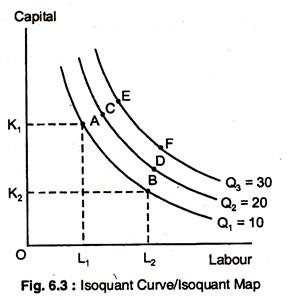
In addition, the isoquant curve can be used to analyze the substitutability and complementarity of inputs. If the isoquant curves are close together, it indicates that the inputs are highly substitutable, meaning that one input can easily be replaced by another. Conversely, if the isoquant curves are far apart, it indicates that the inputs are complementary, meaning that they are used together in fixed proportions.

Overall, the isoquant curve provides valuable insights into the production process and helps firms make informed decisions regarding input allocation and output levels.

Properties of Isoquant Curve

1. Slope of the Isoquant Curve

The slope of the isoquant curve represents the rate at which one input can be substituted for another while keeping the level of output constant. The negative slope indicates that as one input increases, the other must decrease to maintain the same level of output. The steeper the slope, the less substitutable the inputs are.

2. Convex Shape

The isoquant curve is typically convex to the origin, which means that the rate of substitution between inputs is not constant. This convex shape reflects the diminishing marginal rate of technical substitution, indicating that as more of one input is used, larger amounts of the other input are required to maintain the same level of output.

3. Non-Intersecting Isoquant Curves

Each isoquant curve represents a specific level of output. Isoquant curves do not intersect because each curve represents a unique combination of inputs that can produce a specific level of output. If the curves were to intersect, it would imply that the same combination of inputs can produce different levels of output, which is not possible.

4. Isoquant Map

By plotting multiple isoquant curves on a graph, an isoquant map can be created. An isoquant map provides a visual representation of the different combinations of inputs that can produce various levels of output. It allows for the comparison of different production possibilities and helps in determining the optimal combination of inputs for a given level of output.

Formula for Isoquant Curve

An isoquant curve is a graphical representation of all the combinations of inputs that can produce the same level of output. It is a fundamental concept in microeconomics that helps analyze the production possibilities of a firm.

The formula for an isoquant curve is as follows:

Q = f(K, L)

Where:

• Q represents the level of output
• K represents the quantity of capital input
• L represents the quantity of labor input
• f() represents the production function, which shows the relationship between inputs and output

The isoquant curve shows different combinations of capital and labor inputs that can produce the same level of output. Each point on the curve represents a specific combination of inputs. The slope of the isoquant curve represents the rate at which one input can be substituted for another while keeping the level of output constant.

The formula for the isoquant curve allows economists to analyze the efficiency and productivity of a firm. By studying the shape and slope of the curve, economists can determine the optimal combination of inputs that minimizes costs and maximizes output.

In addition, the isoquant curve can be used to analyze the effects of technological advancements and changes in input prices on production. If the shape or position of the curve changes, it indicates a change in the production possibilities of the firm.

Applications of Isoquant Curve in Microeconomics

The isoquant curve is a fundamental concept in microeconomics that has various applications in analyzing production and input combinations. Here are some of the key applications of isoquant curves:

1. Production Analysis: Isoquant curves help in analyzing the different combinations of inputs that can produce a given level of output. By plotting multiple isoquant curves, firms can determine the most efficient input combination for a desired level of output.

2. Input Substitution: Isoquant curves provide insights into the substitutability of inputs in the production process. The slope of the isoquant curve represents the rate at which one input can be substituted for another while keeping the output constant. This information is crucial for firms to make optimal input choices.

3. Cost Minimization: Isoquant curves help firms in minimizing their production costs. By identifying the isoquant curve that represents the desired level of output, firms can determine the input combination that minimizes the cost of production while maintaining the output level.

4. Economies of Scale: Isoquant curves can also be used to analyze economies of scale. By examining the shape and position of the isoquant curves, firms can determine whether they are experiencing increasing, constant, or decreasing returns to scale. This information is useful for firms in making decisions regarding their production scale.

5. Technological Progress: Isoquant curves can be used to analyze the impact of technological progress on production. By comparing isoquant curves over time, firms can assess the changes in input requirements and the potential improvements in production efficiency.

6. Input Pricing: Isoquant curves can help firms in determining the optimal input pricing strategy. By considering the shape and position of the isoquant curves, firms can make decisions regarding the allocation of resources and negotiate input prices to maximize their profits.