The Law Of Supply: The Curve, Types, And Examples

Types of Supply

1. Individual Supply

2. Market Supply

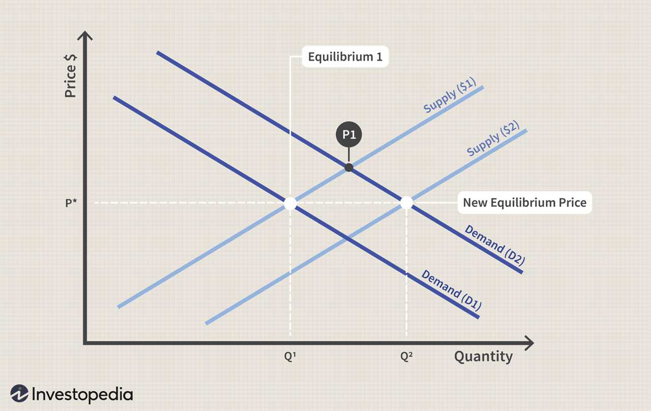
Market supply refers to the total quantity of a good or service that all producers in a market are willing and able to offer for sale at various prices. It is derived by summing up the individual supply curves of all producers in the market. Market supply curves also slope upward, reflecting the positive relationship between price and quantity supplied.

3. Short-Run Supply

Short-run supply refers to the quantity of a good or service that producers are willing and able to offer for sale in the short run, given the existing production capacity and input prices. It takes into account factors that can be adjusted in the short run, such as labor and raw material costs. Short-run supply curves can be upward sloping, downward sloping, or even horizontal, depending on the specific market conditions.

4. Long-Run Supply

Long-run supply refers to the quantity of a good or service that producers are willing and able to offer for sale in the long run, after all factors of production can be adjusted. It considers factors such as capital investments, technological advancements, and changes in market structure. Long-run supply curves are typically upward sloping, indicating that as prices increase, producers have more time to adjust their production processes and increase output.

5. Elastic Supply

Elastic supply refers to a situation where the quantity supplied of a good or service is highly responsive to changes in price. Producers can easily adjust their production levels in response to price changes, resulting in a relatively large change in quantity supplied. Elastic supply curves are flatter, indicating a greater degree of responsiveness to price changes.

6. Inelastic Supply

Inelastic supply refers to a situation where the quantity supplied of a good or service is not very responsive to changes in price. Producers have limited ability to adjust their production levels in the short run, leading to a relatively small change in quantity supplied. Inelastic supply curves are steeper, indicating a lower degree of responsiveness to price changes.

7. Joint Supply

Joint supply refers to a situation where the production of one good or service results in the simultaneous production of another good or service. These goods or services are typically produced together and cannot be easily separated. For example, the production of beef often results in the production of hides as a byproduct. Joint supply curves represent the relationship between the quantities of the two goods or services.

8. Composite Supply

Composite supply refers to a situation where a single good or service is produced using multiple inputs or factors of production. The quantity supplied of the composite good or service depends on the availability and cost of the various inputs. Composite supply curves represent the relationship between the quantity supplied and the prices of the inputs.

Type of Supply	Description	Supply Curve
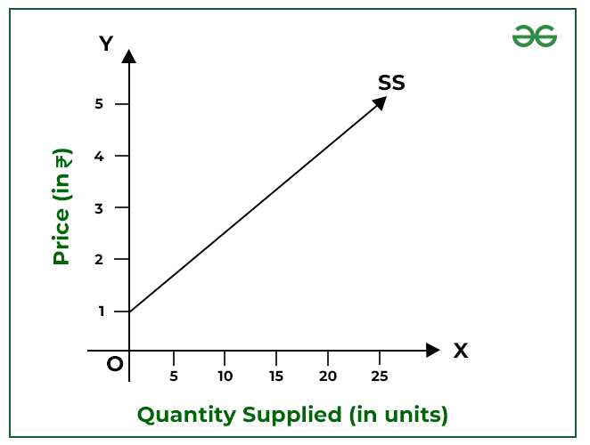
Individual Supply	Quantity supplied by an individual producer at different prices	Upward sloping
Market Supply	Total quantity supplied by all producers in a market at various prices	Upward sloping
Short-Run Supply	Quantity supplied in the short run, given existing production capacity and input prices	Upward, downward, or horizontal sloping
Long-Run Supply	Quantity supplied in the long run, after all factors of production can be adjusted	Upward sloping
Elastic Supply	Highly responsive quantity supplied to price changes	Flatter
Inelastic Supply	Not very responsive quantity supplied to price changes	Steeper
Joint Supply	Simultaneous production of two goods or services	Depends on the specific relationship
Composite Supply	Production of a single good or service using multiple inputs	Depends on the specific relationship

Examples of the Law of Supply

Example 1: Apples

Let’s consider the market for apples. Suppose the price of apples increases due to a decrease in supply caused by a drought that affects apple orchards. As a result, apple farmers are able to sell their apples at a higher price. In response to the higher price, apple farmers may decide to increase their production by planting more apple trees or expanding their existing orchards. This increase in supply leads to a larger quantity of apples being available in the market.

Example 2: Oil

Another example of the law of supply can be seen in the market for oil. When the price of oil rises, oil producers have an incentive to increase their production in order to take advantage of the higher prices. They may invest in new drilling technologies or explore new oil fields to extract more oil. As a result, the quantity of oil supplied to the market increases.

On the other hand, if the price of oil decreases, oil producers may decide to reduce their production as it becomes less profitable. This decrease in supply leads to a smaller quantity of oil being available in the market.

Example 3: Labor Market

The law of supply also applies to the labor market. When wages increase, workers are more likely to enter the workforce or work longer hours. This increase in the supply of labor leads to a larger quantity of workers available for employment.

Conversely, if wages decrease, workers may choose to work fewer hours or seek alternative employment opportunities. This decrease in the supply of labor leads to a smaller quantity of workers available for employment.

Overall, these examples illustrate how the law of supply operates in various markets. As prices increase, producers are incentivized to increase their supply, resulting in a larger quantity of goods or services being available in the market. Conversely, as prices decrease, producers may reduce their supply, leading to a smaller quantity of goods or services being available.